Introduction
The olsrr package provides following tools for teaching and learning OLS regression using R:
- comprehensive regression output
- residual diagnostics
- measures of influence
- heteroskedasticity tests
- collinearity diagnostics
- model fit assessment
- variable contribution assessment
- variable selection procedures
This document is a quickstart guide to the tools offered by olsrr. Other vignettes provide more details on specific topics:
Residual Diagnostics: Includes plots to examine residuals to validate OLS assumptions
Variable selection: Differnt variable selection procedures such as all possible regression, best subset regression, stepwise regression, stepwise forward regression and stepwise backward regression
Heteroskedasticity: Tests for heteroskedasticity include bartlett test, breusch pagan test, score test and f test
Measures of influence: Includes 10 different plots to detect and identify influential observations
Collinearity diagnostics: VIF, Tolerance and condition indices to detect collinearity and plots for assessing mode fit and contributions of variables
Regression
ols_regress(mpg ~ disp + hp + wt + qsec, data = mtcars)## Model Summary
## ---------------------------------------------------------------
## R 0.914 RMSE 2.409
## R-Squared 0.835 MSE 6.875
## Adj. R-Squared 0.811 Coef. Var 13.051
## Pred R-Squared 0.771 AIC 159.070
## MAE 1.858 SBC 167.864
## ---------------------------------------------------------------
## RMSE: Root Mean Square Error
## MSE: Mean Square Error
## MAE: Mean Absolute Error
## AIC: Akaike Information Criteria
## SBC: Schwarz Bayesian Criteria
##
## ANOVA
## --------------------------------------------------------------------
## Sum of
## Squares DF Mean Square F Sig.
## --------------------------------------------------------------------
## Regression 940.412 4 235.103 34.195 0.0000
## Residual 185.635 27 6.875
## Total 1126.047 31
## --------------------------------------------------------------------
##
## Parameter Estimates
## ----------------------------------------------------------------------------------------
## model Beta Std. Error Std. Beta t Sig lower upper
## ----------------------------------------------------------------------------------------
## (Intercept) 27.330 8.639 3.164 0.004 9.604 45.055
## disp 0.003 0.011 0.055 0.248 0.806 -0.019 0.025
## hp -0.019 0.016 -0.212 -1.196 0.242 -0.051 0.013
## wt -4.609 1.266 -0.748 -3.641 0.001 -7.206 -2.012
## qsec 0.544 0.466 0.161 1.166 0.254 -0.413 1.501
## ----------------------------------------------------------------------------------------In the presence of interaction terms in the model, the predictors are
scaled and centered before computing the standardized betas.
ols_regress() will detect interaction terms automatically
but in case you have created a new variable instead of using the inline
function *, you can indicate the presence of interaction
terms by setting iterm to TRUE.
Residual vs Fitted Values Plot
Plot to detect non-linearity, unequal error variances, and outliers.
model <- lm(mpg ~ disp + hp + wt + qsec, data = mtcars)
ols_plot_resid_fit(model)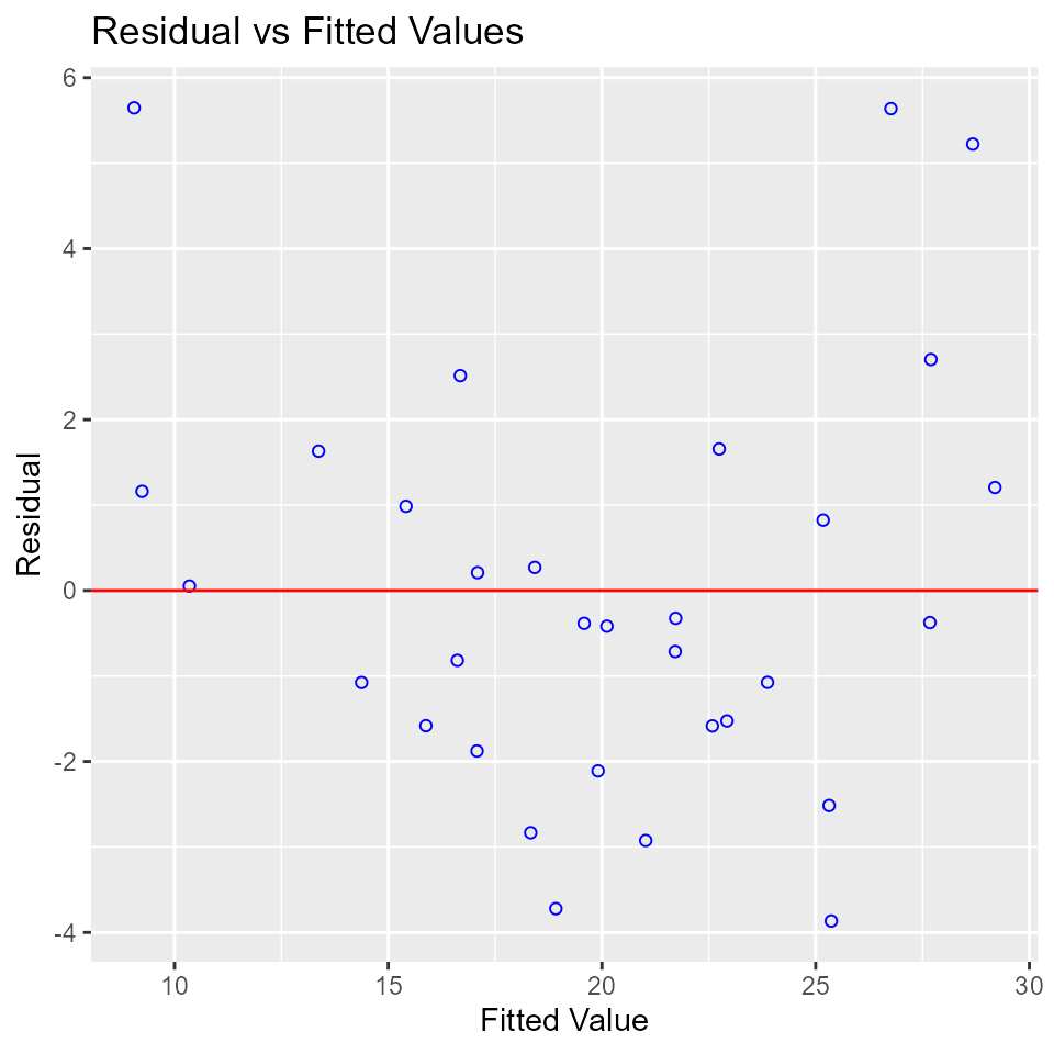
DFBETAs Panel
DFBETAs measure the difference in each parameter estimate with and
without the influential observation. dfbetas_panel creates
plots to detect influential observations using DFBETAs.
model <- lm(mpg ~ disp + hp + wt, data = mtcars)
ols_plot_dfbetas(model)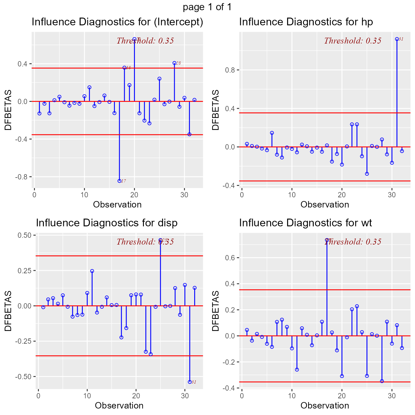
Residual Fit Spread Plot
Plot to detect non-linearity, influential observations and outliers.
model <- lm(mpg ~ disp + hp + wt + qsec, data = mtcars)
ols_plot_resid_fit_spread(model)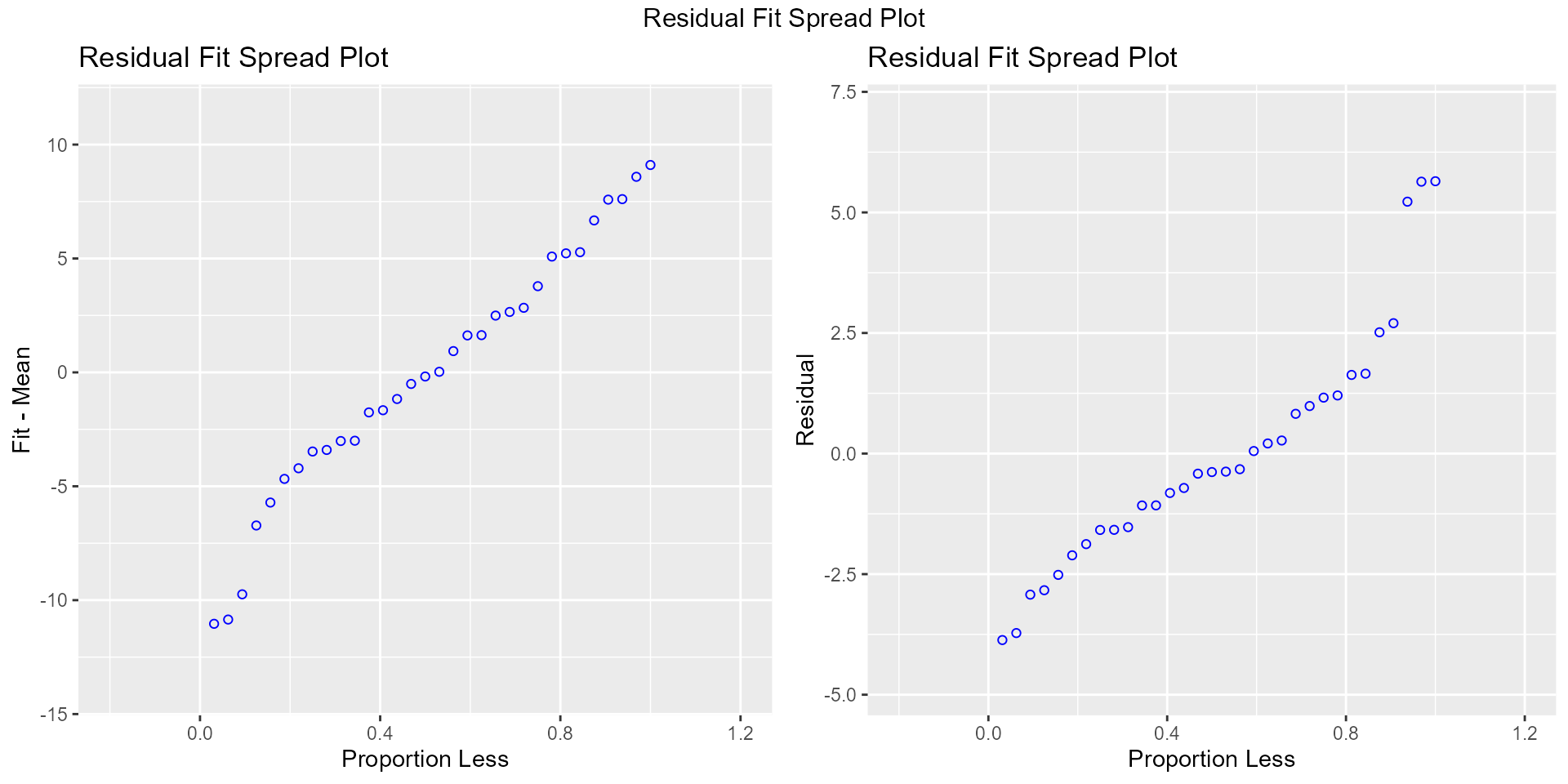
Breusch Pagan Test
Breusch Pagan test is used to test for herteroskedasticity (non-constant error variance). It tests whether the variance of the errors from a regression is dependent on the values of the independent variables. It is a \(\chi^{2}\) test.
model <- lm(mpg ~ disp + hp + wt + drat, data = mtcars)
ols_test_breusch_pagan(model)
##
## Breusch Pagan Test for Heteroskedasticity
## -----------------------------------------
## Ho: the variance is constant
## Ha: the variance is not constant
##
## Data
## -------------------------------
## Response : mpg
## Variables: fitted values of mpg
##
## Test Summary
## ---------------------------
## DF = 1
## Chi2 = 1.429672
## Prob > Chi2 = 0.231818Collinearity Diagnostics
model <- lm(mpg ~ disp + hp + wt + qsec, data = mtcars)
ols_coll_diag(model)
## Tolerance and Variance Inflation Factor
## ---------------------------------------
## Variables Tolerance VIF
## 1 disp 0.1252279 7.985439
## 2 hp 0.1935450 5.166758
## 3 wt 0.1445726 6.916942
## 4 qsec 0.3191708 3.133119
##
##
## Eigenvalue and Condition Index
## ------------------------------
## Eigenvalue Condition Index intercept disp hp wt
## 1 4.721487187 1.000000 0.000123237 0.001132468 0.001413094 0.0005253393
## 2 0.216562203 4.669260 0.002617424 0.036811051 0.027751289 0.0002096014
## 3 0.050416837 9.677242 0.001656551 0.120881424 0.392366164 0.0377028008
## 4 0.010104757 21.616057 0.025805998 0.777260487 0.059594623 0.7017528428
## 5 0.001429017 57.480524 0.969796790 0.063914571 0.518874831 0.2598094157
## qsec
## 1 0.0001277169
## 2 0.0046789491
## 3 0.0001952599
## 4 0.0024577686
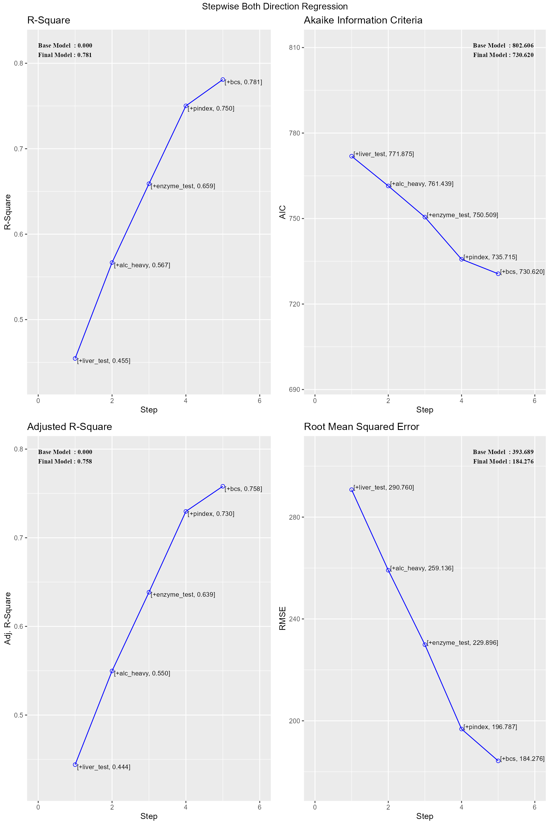
## 5 0.9925403056Stepwise Regression
Build regression model from a set of candidate predictor variables by entering and removing predictors based on p values, in a stepwise manner until there is no variable left to enter or remove any more.
Variable Selection
# stepwise regression
model <- lm(y ~ ., data = surgical)
ols_step_both_p(model)
##
##
## Stepwise Summary
## ------------------------------------------------------------------------------
## Step Variable AIC SBC SBIC R2 Adj. R2
## ------------------------------------------------------------------------------
## 0 Base Model 802.606 806.584 646.794 0.00000 0.00000
## 1 liver_test (+) 771.875 777.842 616.009 0.45454 0.44405
## 2 alc_heavy (+) 761.439 769.395 605.506 0.56674 0.54975
## 3 enzyme_test (+) 750.509 760.454 595.297 0.65900 0.63854
## 4 pindex (+) 735.715 747.649 582.943 0.75015 0.72975
## 5 bcs (+) 730.620 744.543 579.638 0.78091 0.75808
## ------------------------------------------------------------------------------
##
## Final Model Output
## ------------------
##
## Model Summary
## -------------------------------------------------------------------
## R 0.884 RMSE 184.276
## R-Squared 0.781 MSE 38202.426
## Adj. R-Squared 0.758 Coef. Var 27.839
## Pred R-Squared 0.700 AIC 730.620
## MAE 137.656 SBC 744.543
## -------------------------------------------------------------------
## RMSE: Root Mean Square Error
## MSE: Mean Square Error
## MAE: Mean Absolute Error
## AIC: Akaike Information Criteria
## SBC: Schwarz Bayesian Criteria
##
## ANOVA
## -----------------------------------------------------------------------
## Sum of
## Squares DF Mean Square F Sig.
## -----------------------------------------------------------------------
## Regression 6535804.090 5 1307160.818 34.217 0.0000
## Residual 1833716.447 48 38202.426
## Total 8369520.537 53
## -----------------------------------------------------------------------
##
## Parameter Estimates
## ------------------------------------------------------------------------------------------------
## model Beta Std. Error Std. Beta t Sig lower upper
## ------------------------------------------------------------------------------------------------
## (Intercept) -1178.330 208.682 -5.647 0.000 -1597.914 -758.746
## liver_test 58.064 40.144 0.156 1.446 0.155 -22.652 138.779
## alc_heavy 317.848 71.634 0.314 4.437 0.000 173.818 461.878
## enzyme_test 9.748 1.656 0.521 5.887 0.000 6.419 13.077
## pindex 8.924 1.808 0.380 4.935 0.000 5.288 12.559
## bcs 59.864 23.060 0.241 2.596 0.012 13.498 106.230
## ------------------------------------------------------------------------------------------------
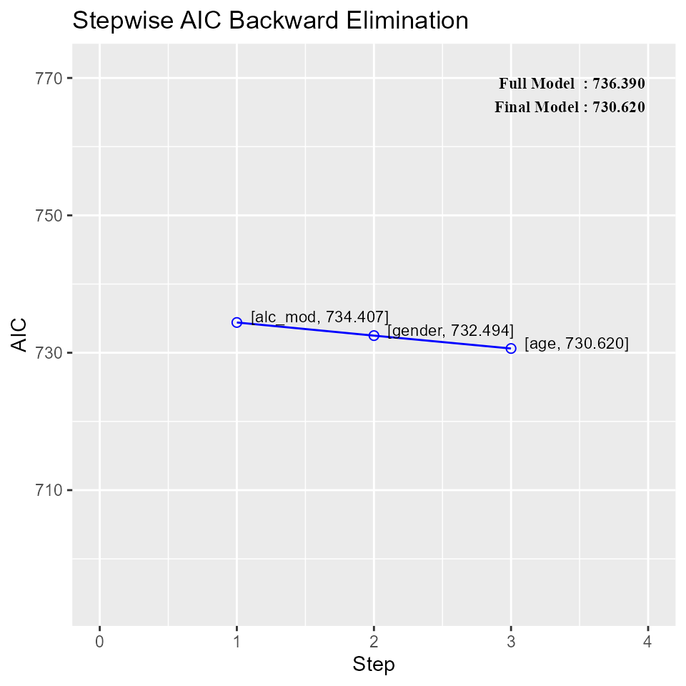
Stepwise AIC Backward Regression
Build regression model from a set of candidate predictor variables by removing predictors based on Akaike Information Criteria, in a stepwise manner until there is no variable left to remove any more.
Variable Selection
# stepwise aic backward regression
model <- lm(y ~ ., data = surgical)
k <- ols_step_backward_aic(model)
k
##
##
## Stepwise Summary
## -------------------------------------------------------------------------
## Step Variable AIC SBC SBIC R2 Adj. R2
## -------------------------------------------------------------------------
## 0 Full Model 736.390 756.280 586.665 0.78184 0.74305
## 1 alc_mod 734.407 752.308 583.884 0.78177 0.74856
## 2 gender 732.494 748.406 581.290 0.78142 0.75351
## 3 age 730.620 744.543 578.844 0.78091 0.75808
## -------------------------------------------------------------------------
##
## Final Model Output
## ------------------
##
## Model Summary
## -------------------------------------------------------------------
## R 0.884 RMSE 184.276
## R-Squared 0.781 MSE 38202.426
## Adj. R-Squared 0.758 Coef. Var 27.839
## Pred R-Squared 0.700 AIC 730.620
## MAE 137.656 SBC 744.543
## -------------------------------------------------------------------
## RMSE: Root Mean Square Error
## MSE: Mean Square Error
## MAE: Mean Absolute Error
## AIC: Akaike Information Criteria
## SBC: Schwarz Bayesian Criteria
##
## ANOVA
## -----------------------------------------------------------------------
## Sum of
## Squares DF Mean Square F Sig.
## -----------------------------------------------------------------------
## Regression 6535804.090 5 1307160.818 34.217 0.0000
## Residual 1833716.447 48 38202.426
## Total 8369520.537 53
## -----------------------------------------------------------------------
##
## Parameter Estimates
## ------------------------------------------------------------------------------------------------
## model Beta Std. Error Std. Beta t Sig lower upper
## ------------------------------------------------------------------------------------------------
## (Intercept) -1178.330 208.682 -5.647 0.000 -1597.914 -758.746
## bcs 59.864 23.060 0.241 2.596 0.012 13.498 106.230
## pindex 8.924 1.808 0.380 4.935 0.000 5.288 12.559
## enzyme_test 9.748 1.656 0.521 5.887 0.000 6.419 13.077
## liver_test 58.064 40.144 0.156 1.446 0.155 -22.652 138.779
## alc_heavy 317.848 71.634 0.314 4.437 0.000 173.818 461.878
## ------------------------------------------------------------------------------------------------