Residual plus component plot

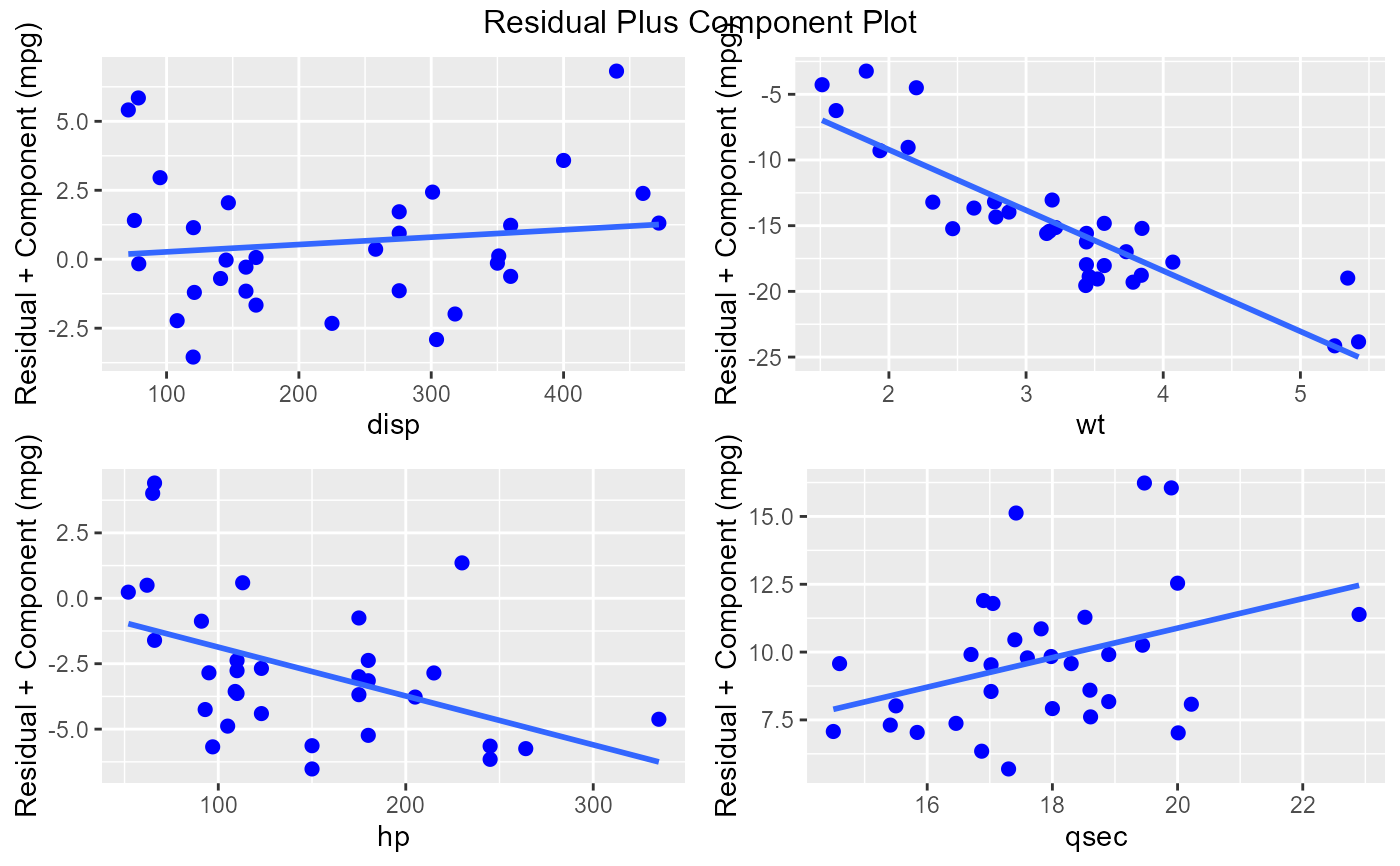
The residual plus component plot indicates whether any non-linearity is present in the relationship between response and predictor variables and can suggest possible transformations for linearizing the data.

Usage

ols_plot_comp_plus_resid(model, print_plot = TRUE)

Arguments

model

An object of class lm.

print_plot

logical; if TRUE, prints the plot else returns a plot object.

References

Chatterjee, Samprit and Hadi, Ali. Regression Analysis by Example. 5th ed. N.p.: John Wiley & Sons, 2012. Print.

Kutner, MH, Nachtscheim CJ, Neter J and Li W., 2004, Applied Linear Statistical Models (5th edition). Chicago, IL., McGraw Hill/Irwin.

See also

ols_plot_added_variable(), ols_plot_resid_regressor()

Examples

model <- lm(mpg ~ disp + hp + wt + qsec, data = mtcars)
ols_plot_comp_plus_resid(model)
#> `geom_smooth()` using formula = 'y ~ x'
#> `geom_smooth()` using formula = 'y ~ x'
#> `geom_smooth()` using formula = 'y ~ x'
#> `geom_smooth()` using formula = 'y ~ x'