Fits all regressions involving one regressor, two regressors, three regressors, and so on. It tests all possible subsets of the set of potential independent variables.
Usage
ols_step_all_possible(model, ...)

# Default S3 method
ols_step_all_possible(model, max_order = NULL, force = FALSE, ...)

# S3 method for class 'ols_step_all_possible'
plot(x, model = NA, print_plot = TRUE, ...)
Arguments
- model
An object of class
lm.- ...
Other arguments.
- max_order
Maximum subset order.
- force
logical; if
TRUE, allows the combinatorial subset search to proceed when more than2^20 - 1models would be fitted.- x
An object of class
ols_step_all_possible.- print_plot
logical; if
TRUE, prints the plot else returns a plot object.
Value
ols_step_all_possible returns an object of class "ols_step_all_possible".
An object of class "ols_step_all_possible" is a data frame containing the
following components:
- mindex
model index
- n
number of predictors
- predictors
predictors in the model
- rsquare
rsquare of the model
- adjr
adjusted rsquare of the model
- rmse
root mean squared error of the model
- predrsq
predicted rsquare of the model
- cp
mallow's Cp
- aic
akaike information criteria
- sbic
sawa bayesian information criteria
- sbc
schwarz bayes information criteria
- msep
estimated MSE of prediction, assuming multivariate normality
- fpe
final prediction error
- apc
amemiya prediction criteria
- hsp
hocking's Sp
Details
Refits accept explicit contrast matrices or the base contrast names
contr.treatment, contr.sum, contr.helmert, contr.poly and contr.SAS
(resolved from the stats namespace); models fitted with custom named contrast
functions must be refitted with an explicit matrix, for example
contrasts = list(g = my_matrix). Refits carry the fitted model's frozen total
offset as an argument with all formula offset() terms removed for
standardized-beta and selection computations. Returned stepwise models are
fitted from the original call, preserving formula and argument offsets for
prediction on new data. Their coefficients, fitted values and total offset
must be identical to the frozen-offset selection fit; otherwise selection
stops with an error because prediction with new data is not supported for
that model.
For non-hierarchical stepwise selection, candidate rankings and criterion improvement tests use 10 significant digits: values that agree to 10 significant digits are ties, equal criterion values mean no improvement, and a remaining tie goes to the first candidate in formula order after any F tie is broken by p value (smaller for entry, larger for removal). P-value entry and removal cutoffs are compared without rounding.
References
Mendenhall William and Sinsich Terry, 2012, A Second Course in Statistics Regression Analysis (7th edition). Prentice Hall
Examples
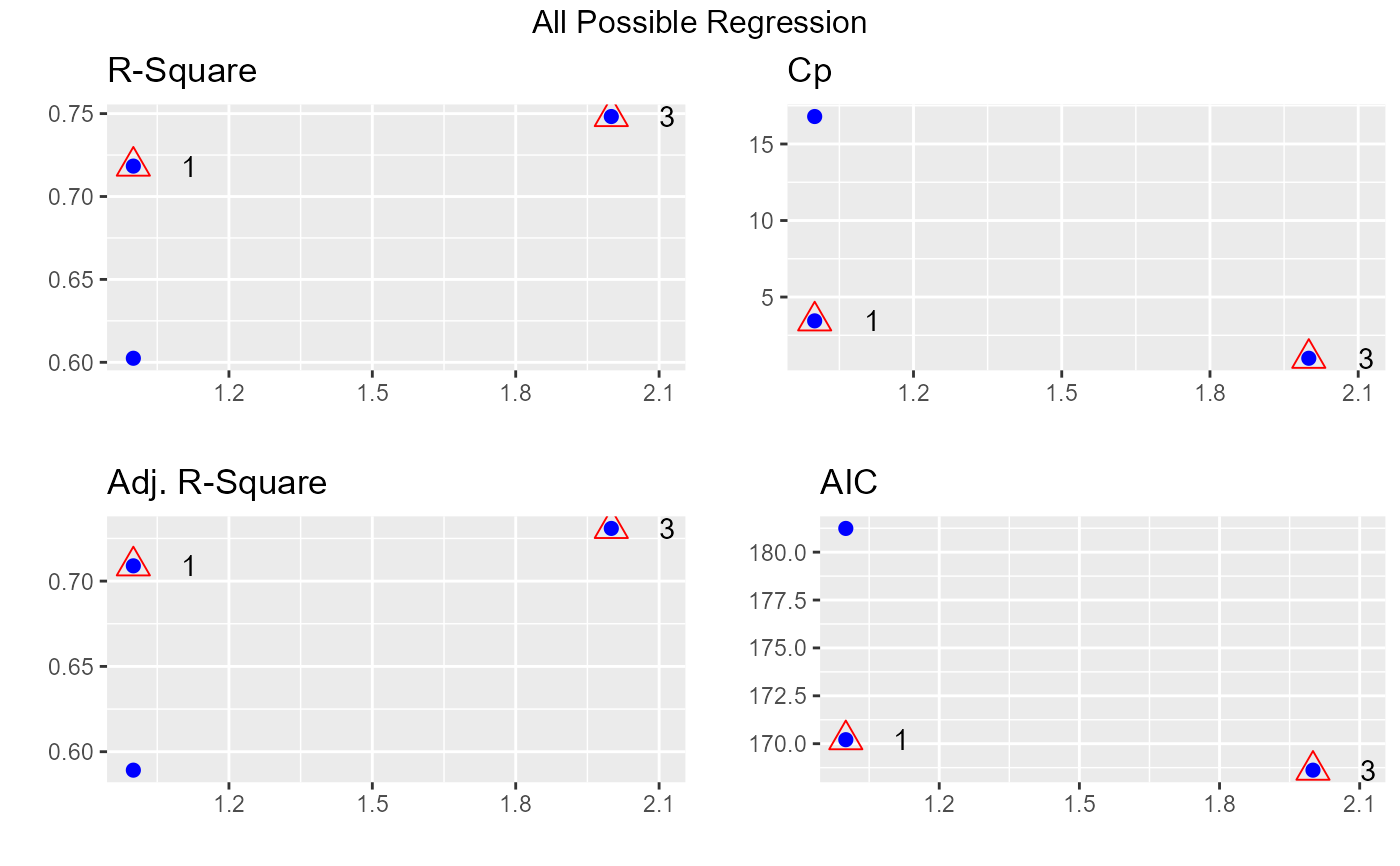
model <- lm(mpg ~ disp + hp, data = mtcars)
k <- ols_step_all_possible(model)
k
#> Index N Predictors R-Square Adj. R-Square Mallow's Cp
#> 1 1 1 disp 0.7183433 0.7089548 4.443792
#> 2 2 1 hp 0.6024373 0.5891853 17.794906
#> 3 3 2 disp hp 0.7482402 0.7308774 3.000000
# plot
plot(k)
 # maximum subset
model <- lm(mpg ~ disp + hp + drat + wt + qsec, data = mtcars)
ols_step_all_possible(model, max_order = 3)
#> Index N Predictors R-Square Adj. R-Square Mallow's Cp
#> 4 1 1 wt 0.7528328 0.7445939 14.534575
#> 1 2 1 disp 0.7183433 0.7089548 20.469805
#> 2 3 1 hp 0.6024373 0.5891853 40.415867
#> 3 4 1 drat 0.4639952 0.4461283 64.240140
#> 5 5 1 qsec 0.1752963 0.1478062 113.921823
#> 11 6 2 hp wt 0.8267855 0.8148396 3.808191
#> 15 7 2 wt qsec 0.8264161 0.8144448 3.871747
#> 8 8 2 disp wt 0.7809306 0.7658223 11.699275
#> 13 9 2 drat wt 0.7608970 0.7444071 15.146825
#> 6 10 2 disp hp 0.7482402 0.7308774 17.324909
#> 10 11 2 hp drat 0.7411716 0.7233214 18.541329
#> 7 12 2 disp drat 0.7310094 0.7124583 20.290124
#> 9 13 2 disp qsec 0.7215598 0.7023571 21.916283
#> 12 14 2 hp qsec 0.6368769 0.6118339 36.489228
#> 14 15 2 drat qsec 0.5921951 0.5640706 44.178433
#> 25 16 3 drat wt qsec 0.8370214 0.8195594 4.046701
#> 22 17 3 hp drat wt 0.8368791 0.8194018 4.071201
#> 24 18 3 hp wt qsec 0.8347678 0.8170643 4.434529
#> 17 19 3 disp hp wt 0.8268361 0.8082829 5.799467
#> 21 20 3 disp wt qsec 0.8264170 0.8078189 5.871590
#> 19 21 3 disp drat wt 0.7835315 0.7603385 13.251685
#> 16 22 3 disp hp drat 0.7750131 0.7509073 14.717610
#> 18 23 3 disp hp qsec 0.7541953 0.7278591 18.300105
#> 23 24 3 hp drat qsec 0.7442512 0.7168495 20.011366
#> 20 25 3 disp drat qsec 0.7412673 0.7135459 20.524864