Select the subset of predictors that do the best at meeting some well-defined objective criterion, such as having the largest R2 value or the smallest MSE, Mallow's Cp or AIC. The default metric used for selecting the model is R2 but the user can choose any of the other available metrics.
Usage
ols_step_best_subset(model, ...)

# Default S3 method
ols_step_best_subset(
  model,
  max_order = NULL,
  include = NULL,
  exclude = NULL,
  metric = c("rsquare", "adjr", "predrsq", "cp", "aic", "sbic", "sbc", "msep", "fpe",
    "apc", "hsp"),
  ...
)

# S3 method for class 'ols_step_best_subset'
plot(x, model = NA, print_plot = TRUE, ...)
Arguments
- model
An object of class
lm.- ...
Other inputs.
- max_order
Maximum subset order.
- include
Character or numeric vector; variables to be included in selection process.
- exclude
Character or numeric vector; variables to be excluded from selection process.
- metric
Metric to select model.
- x
An object of class
ols_step_best_subset.- print_plot
logical; if
TRUE, prints the plot else returns a plot object.
Value
ols_step_best_subset returns an object of class "ols_step_best_subset".
An object of class "ols_step_best_subset" is a list containing the following:
- metrics
selection metrics
Details
Refits accept explicit contrast matrices or the base contrast names
contr.treatment, contr.sum, contr.helmert, contr.poly and contr.SAS
(resolved from the stats namespace); models fitted with custom named contrast
functions must be refitted with an explicit matrix, for example
contrasts = list(g = my_matrix). Refits carry the fitted model's frozen total
offset as an argument with all formula offset() terms removed for
standardized-beta and selection computations. Returned stepwise models are
fitted from the original call, preserving formula and argument offsets for
prediction on new data. Their coefficients, fitted values and total offset
must be identical to the frozen-offset selection fit; otherwise selection
stops with an error because prediction with new data is not supported for
that model.
For non-hierarchical stepwise selection, candidate rankings and criterion improvement tests use 10 significant digits: values that agree to 10 significant digits are ties, equal criterion values mean no improvement, and a remaining tie goes to the first candidate in formula order after any F tie is broken by p value (smaller for entry, larger for removal). P-value entry and removal cutoffs are compared without rounding.
References
Kutner, MH, Nachtscheim CJ, Neter J and Li W., 2004, Applied Linear Statistical Models (5th edition). Chicago, IL., McGraw Hill/Irwin.
Examples
model <- lm(mpg ~ disp + hp + wt + qsec, data = mtcars)
ols_step_best_subset(model)
#> Best Subsets Regression
#> ------------------------------
#> Model Index Predictors
#> ------------------------------
#> 1 wt
#> 2 hp wt
#> 3 hp wt qsec
#> 4 disp hp wt qsec
#> ------------------------------
#>
#> Subsets Regression Summary
#> -------------------------------------------------------------------------------------------------------------------------------
#> Adj. Pred
#> Model R-Square R-Square R-Square C(p) AIC SBIC SBC MSEP FPE HSP APC
#> -------------------------------------------------------------------------------------------------------------------------------
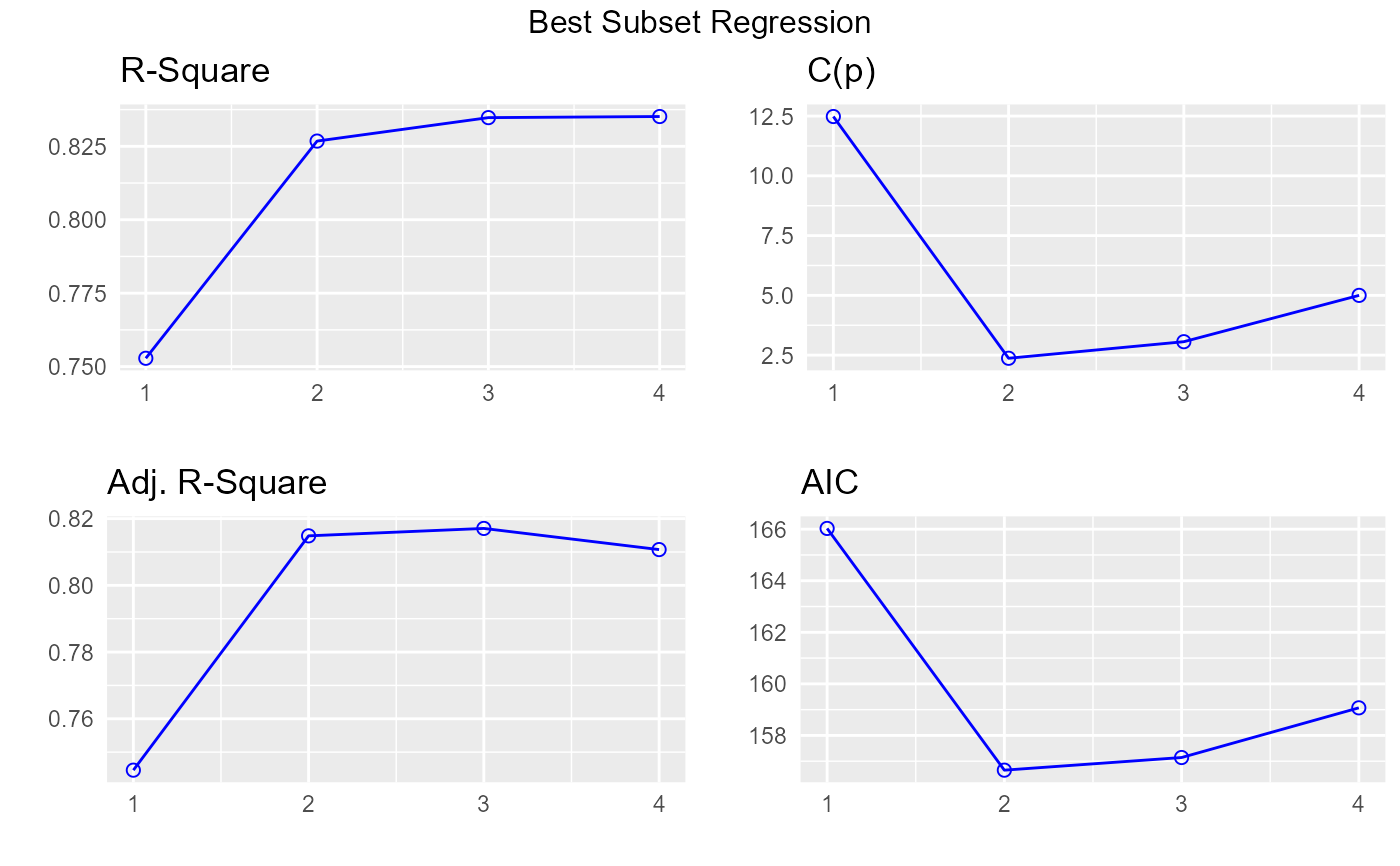
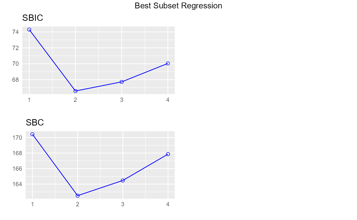
#> 1 0.7528 0.7446 0.7087 12.4809 166.0294 74.2916 170.4266 9.8972 9.8572 0.3199 0.2801
#> 2 0.8268 0.8148 0.7811 2.3690 156.6523 66.5755 162.5153 7.4314 7.3563 0.2402 0.2091
#> 3 0.8348 0.8171 0.782 3.0617 157.1426 67.7238 164.4713 7.6140 7.4756 0.2461 0.2124
#> 4 0.8351 0.8107 0.771 5.0000 159.0696 70.0408 167.8640 8.1810 7.9497 0.2644 0.2259
#> -------------------------------------------------------------------------------------------------------------------------------
#> AIC: Akaike Information Criteria
#> SBIC: Sawa's Bayesian Information Criteria
#> SBC: Schwarz Bayesian Criteria
#> MSEP: Estimated error of prediction, assuming multivariate normality
#> FPE: Final Prediction Error
#> HSP: Hocking's Sp
#> APC: Amemiya Prediction Criteria
#>
ols_step_best_subset(model, metric = "adjr")
#> Best Subsets Regression
#> ------------------------------
#> Model Index Predictors
#> ------------------------------
#> 1 wt
#> 2 hp wt
#> 3 hp wt qsec
#> 4 disp hp wt qsec
#> ------------------------------
#>
#> Subsets Regression Summary
#> -------------------------------------------------------------------------------------------------------------------------------
#> Adj. Pred
#> Model R-Square R-Square R-Square C(p) AIC SBIC SBC MSEP FPE HSP APC
#> -------------------------------------------------------------------------------------------------------------------------------
#> 1 0.7528 0.7446 0.7087 12.4809 166.0294 74.2916 170.4266 9.8972 9.8572 0.3199 0.2801
#> 2 0.8268 0.8148 0.7811 2.3690 156.6523 66.5755 162.5153 7.4314 7.3563 0.2402 0.2091
#> 3 0.8348 0.8171 0.782 3.0617 157.1426 67.7238 164.4713 7.6140 7.4756 0.2461 0.2124
#> 4 0.8351 0.8107 0.771 5.0000 159.0696 70.0408 167.8640 8.1810 7.9497 0.2644 0.2259
#> -------------------------------------------------------------------------------------------------------------------------------
#> AIC: Akaike Information Criteria
#> SBIC: Sawa's Bayesian Information Criteria
#> SBC: Schwarz Bayesian Criteria
#> MSEP: Estimated error of prediction, assuming multivariate normality
#> FPE: Final Prediction Error
#> HSP: Hocking's Sp
#> APC: Amemiya Prediction Criteria
#>
ols_step_best_subset(model, metric = "cp")
#> Best Subsets Regression
#> ------------------------------
#> Model Index Predictors
#> ------------------------------
#> 1 wt
#> 2 hp wt
#> 3 hp wt qsec
#> 4 disp hp wt qsec
#> ------------------------------
#>
#> Subsets Regression Summary
#> -------------------------------------------------------------------------------------------------------------------------------
#> Adj. Pred
#> Model R-Square R-Square R-Square C(p) AIC SBIC SBC MSEP FPE HSP APC
#> -------------------------------------------------------------------------------------------------------------------------------
#> 1 0.7528 0.7446 0.7087 12.4809 166.0294 74.2916 170.4266 9.8972 9.8572 0.3199 0.2801
#> 2 0.8268 0.8148 0.7811 2.3690 156.6523 66.5755 162.5153 7.4314 7.3563 0.2402 0.2091
#> 3 0.8348 0.8171 0.782 3.0617 157.1426 67.7238 164.4713 7.6140 7.4756 0.2461 0.2124
#> 4 0.8351 0.8107 0.771 5.0000 159.0696 70.0408 167.8640 8.1810 7.9497 0.2644 0.2259
#> -------------------------------------------------------------------------------------------------------------------------------
#> AIC: Akaike Information Criteria
#> SBIC: Sawa's Bayesian Information Criteria
#> SBC: Schwarz Bayesian Criteria
#> MSEP: Estimated error of prediction, assuming multivariate normality
#> FPE: Final Prediction Error
#> HSP: Hocking's Sp
#> APC: Amemiya Prediction Criteria
#>
# maximum subset
model <- lm(mpg ~ disp + hp + drat + wt + qsec, data = mtcars)
ols_step_best_subset(model, max_order = 3)
#> Best Subsets Regression
#> ---------------------------
#> Model Index Predictors
#> ---------------------------
#> 1 wt
#> 2 hp wt
#> 3 drat wt qsec
#> ---------------------------
#>
#> Subsets Regression Summary
#> -------------------------------------------------------------------------------------------------------------------------------
#> Adj. Pred
#> Model R-Square R-Square R-Square C(p) AIC SBIC SBC MSEP FPE HSP APC
#> -------------------------------------------------------------------------------------------------------------------------------
#> 1 0.7528 0.7446 0.7087 14.5346 166.0294 74.1040 170.4266 9.8972 9.8572 0.3199 0.2801
#> 2 0.8268 0.8148 0.7811 3.8082 156.6523 66.2706 162.5153 7.4314 7.3563 0.2402 0.2091
#> 3 0.8370 0.8196 0.7765 4.0467 156.7031 66.9790 164.0318 7.5102 7.3736 0.2428 0.2095
#> -------------------------------------------------------------------------------------------------------------------------------
#> AIC: Akaike Information Criteria
#> SBIC: Sawa's Bayesian Information Criteria
#> SBC: Schwarz Bayesian Criteria
#> MSEP: Estimated error of prediction, assuming multivariate normality
#> FPE: Final Prediction Error
#> HSP: Hocking's Sp
#> APC: Amemiya Prediction Criteria
#>
# plot
model <- lm(mpg ~ disp + hp + wt + qsec, data = mtcars)
k <- ols_step_best_subset(model)
plot(k)
 # return only models including `qsec`
ols_step_best_subset(model, include = c("qsec"))
#> Best Subsets Regression
#> ------------------------------
#> Model Index Predictors
#> ------------------------------
#> 1 qsec
#> 2 qsec wt
#> 3 qsec hp wt
#> 4 qsec disp hp wt
#> ------------------------------
#>
#> Subsets Regression Summary
#> -----------------------------------------------------------------------------------------------------------------------------------
#> Adj. Pred
#> Model R-Square R-Square R-Square C(p) AIC SBIC SBC MSEP FPE HSP APC
#> -----------------------------------------------------------------------------------------------------------------------------------
#> 1 0.1753 0.1478 0.0754 107.0696 204.5881 109.5591 208.9853 33.0233 32.8899 1.0674 0.9347
#> 2 0.8264 0.8144 0.7786 2.4295 156.7205 66.6304 162.5834 7.4472 7.3720 0.2407 0.2095
#> 3 0.8348 0.8171 0.782 3.0617 157.1426 67.7238 164.4713 7.6140 7.4756 0.2461 0.2124
#> 4 0.8351 0.8107 0.771 5.0000 159.0696 70.0408 167.8640 8.1810 7.9497 0.2644 0.2259
#> -----------------------------------------------------------------------------------------------------------------------------------
#> AIC: Akaike Information Criteria
#> SBIC: Sawa's Bayesian Information Criteria
#> SBC: Schwarz Bayesian Criteria
#> MSEP: Estimated error of prediction, assuming multivariate normality
#> FPE: Final Prediction Error
#> HSP: Hocking's Sp
#> APC: Amemiya Prediction Criteria
#>
# exclude `hp` from selection process
ols_step_best_subset(model, exclude = c("hp"))
#> Best Subsets Regression
#> ---------------------------
#> Model Index Predictors
#> ---------------------------
#> 1 wt
#> 2 wt qsec
#> 3 disp wt qsec
#> ---------------------------
#>
#> Subsets Regression Summary
#> -------------------------------------------------------------------------------------------------------------------------------
#> Adj. Pred
#> Model R-Square R-Square R-Square C(p) AIC SBIC SBC MSEP FPE HSP APC
#> -------------------------------------------------------------------------------------------------------------------------------
#> 1 0.7528 0.7446 0.7087 12.4809 166.0294 74.2916 170.4266 9.8972 9.8572 0.3199 0.2801
#> 2 0.8264 0.8144 0.7786 2.4295 156.7205 66.6304 162.5834 7.4472 7.3720 0.2407 0.2095
#> 3 0.8264 0.8078 0.7699 4.4293 158.7203 68.8815 166.0490 7.9988 7.8534 0.2585 0.2232
#> -------------------------------------------------------------------------------------------------------------------------------
#> AIC: Akaike Information Criteria
#> SBIC: Sawa's Bayesian Information Criteria
#> SBC: Schwarz Bayesian Criteria
#> MSEP: Estimated error of prediction, assuming multivariate normality
#> FPE: Final Prediction Error
#> HSP: Hocking's Sp
#> APC: Amemiya Prediction Criteria
#>