Stepwise Adjusted R-Squared regression

Build regression model from a set of candidate predictor variables by entering and removing predictors based on adjusted r-squared, in a stepwise manner until there is no variable left to enter or remove any more.

Usage

ols_step_both_adj_r2(model, ...)

# Default S3 method
ols_step_both_adj_r2(
  model,
  include = NULL,
  exclude = NULL,
  progress = FALSE,
  details = FALSE,
  ...
)

# S3 method for class 'ols_step_both_adj_r2'
plot(x, print_plot = TRUE, details = TRUE, digits = 3, ...)

Arguments

model

An object of class lm.

...

Other arguments.

include

Character or numeric vector; variables to be included in selection process.

exclude

Character or numeric vector; variables to be excluded from selection process.

progress

Logical; if TRUE, will display variable selection progress.

details

Logical; if TRUE, details of variable selection will be printed on screen.

x

An object of class ols_step_both_*.

print_plot

logical; if TRUE, prints the plot else returns a plot object.

digits

Number of decimal places to display.

Value

List containing the following components:

model

final model; an object of class lm

metrics

selection metrics

others

list; info used for plotting and printing

References

Venables, W. N. and Ripley, B. D. (2002) Modern Applied Statistics with S. Fourth edition. Springer.

See also

Other both direction selection procedures: ols_step_both_aic(), ols_step_both_r2(), ols_step_both_sbc(), ols_step_both_sbic()

Examples

if (FALSE) { # \dontrun{
# stepwise regression
model <- lm(y ~ ., data = stepdata)
ols_step_both_adj_r2(model)

# stepwise regression plot
model <- lm(y ~ ., data = stepdata)
k <- ols_step_both_adj_r2(model)
plot(k)

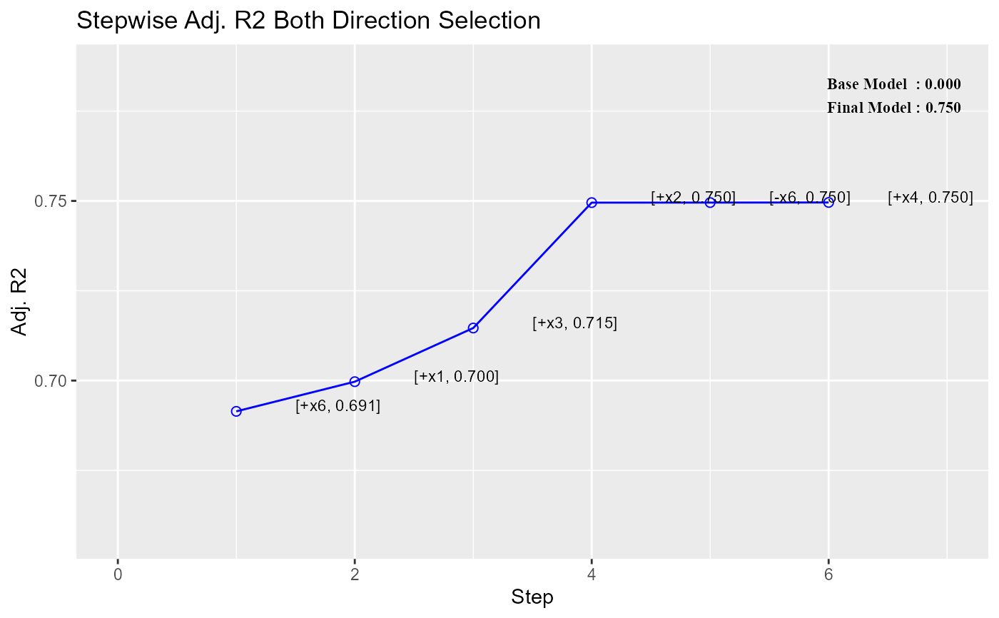# selection metrics
k$metrics

# final model
k$model

# include or exclude variables
# force variable to be included in selection process
model <- lm(y ~ ., data = stepdata)

ols_step_both_adj_r2(model, include = c("x6"))

# use index of variable instead of name
ols_step_both_adj_r2(model, include = c(6))

# force variable to be excluded from selection process
ols_step_both_adj_r2(model, exclude = c("x2"))

# use index of variable instead of name
ols_step_both_adj_r2(model, exclude = c(2))

# include & exclude variables in the selection process
ols_step_both_adj_r2(model, include = c("x6"), exclude = c("x2"))

# use index of variable instead of name
ols_step_both_adj_r2(model, include = c(6), exclude = c(2))
} # }