Build regression model from a set of candidate predictor variables by entering predictors based on p values, in a stepwise manner until there is no variable left to enter any more.
Usage
ols_step_forward_p(model, ...)

# Default S3 method
ols_step_forward_p(
  model,
  p_val = 0.3,
  include = NULL,
  exclude = NULL,
  hierarchical = FALSE,
  progress = FALSE,
  details = FALSE,
  steps = NULL,
  ...
)

# S3 method for class 'ols_step_forward_p'
plot(x, model = NA, print_plot = TRUE, details = TRUE, ...)
Arguments
- model
An object of class
lm; the model should include all candidate predictor variables.- ...
Other arguments.
- p_val
p value; variables with p value less than
p_valwill enter into the model- include
Character or numeric vector; variables to be included in selection process.
- exclude
Character or numeric vector; variables to be excluded from selection process.
- hierarchical
Logical; if
TRUE, performs hierarchical selection.- progress
Logical; if
TRUE, will display variable selection progress.- details
Logical; if
TRUE, will print the regression result at each step.- steps
Number of steps after which the stepwise procedures should stop.
- x
An object of class
ols_step_forward_p.- print_plot
logical; if
TRUE, prints the plot else returns a plot object.
Value
ols_step_forward_p returns an object of class "ols_step_forward_p".
An object of class "ols_step_forward_p" is a list containing the
following components:
- model
final model; an object of class
lm- metrics
selection metrics
Details
Refits accept explicit contrast matrices or the base contrast names
contr.treatment, contr.sum, contr.helmert, contr.poly and contr.SAS
(resolved from the stats namespace); models fitted with custom named contrast
functions must be refitted with an explicit matrix, for example
contrasts = list(g = my_matrix). Refits carry the fitted model's frozen total
offset as an argument with all formula offset() terms removed for
standardized-beta and selection computations. Returned stepwise models are
fitted from the original call, preserving formula and argument offsets for
prediction on new data. Their coefficients, fitted values and total offset
must be identical to the frozen-offset selection fit; otherwise selection
stops with an error because prediction with new data is not supported for
that model.
For non-hierarchical stepwise selection, candidate rankings and criterion improvement tests use 10 significant digits: values that agree to 10 significant digits are ties, equal criterion values mean no improvement, and a remaining tie goes to the first candidate in formula order after any F tie is broken by p value (smaller for entry, larger for removal). P-value entry and removal cutoffs are compared without rounding.
References
Chatterjee, Samprit and Hadi, Ali. Regression Analysis by Example. 5th ed. N.p.: John Wiley & Sons, 2012. Print.
Kutner, MH, Nachtscheim CJ, Neter J and Li W., 2004, Applied Linear Statistical Models (5th edition). Chicago, IL., McGraw Hill/Irwin.
See also
Other forward selection procedures:
ols_step_forward_adj_r2(),
ols_step_forward_aic(),
ols_step_forward_r2(),
ols_step_forward_sbc(),
ols_step_forward_sbic()
Examples
# stepwise forward regression
model <- lm(y ~ ., data = surgical)
ols_step_forward_p(model)
#>
#>
#> Stepwise Summary
#> --------------------------------------------------------------------------
#> Step Variable AIC SBC SBIC R2 Adj. R2
#> --------------------------------------------------------------------------
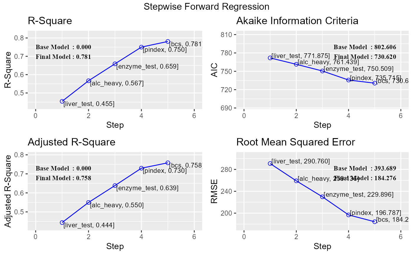
#> 0 Base Model 802.606 806.584 646.794 0.00000 0.00000
#> 1 liver_test 771.875 777.842 616.009 0.45454 0.44405
#> 2 alc_heavy 761.439 769.395 605.506 0.56674 0.54975
#> 3 enzyme_test 750.509 760.454 595.297 0.65900 0.63854
#> 4 pindex 735.715 747.649 582.943 0.75015 0.72975
#> 5 bcs 730.620 744.543 579.638 0.78091 0.75808
#> --------------------------------------------------------------------------
#>
#> Final Model Output
#> ------------------
#>
#> Model Summary
#> -------------------------------------------------------------------
#> R 0.884 RMSE 195.454
#> R-Squared 0.781 MSE 38202.426
#> Adj. R-Squared 0.758 Coef. Var 27.839
#> Pred R-Squared 0.700 AIC 730.620
#> MAE 137.656 SBC 744.543
#> -------------------------------------------------------------------
#> RMSE: Root Mean Square Error
#> MSE: Mean Square Error
#> MAE: Mean Absolute Error
#> AIC: Akaike Information Criteria
#> SBC: Schwarz Bayesian Criteria
#>
#> ANOVA
#> -----------------------------------------------------------------------
#> Sum of
#> Squares DF Mean Square F Sig.
#> -----------------------------------------------------------------------
#> Regression 6535804.090 5 1307160.818 34.217 0.0000
#> Residual 1833716.447 48 38202.426
#> Total 8369520.537 53
#> -----------------------------------------------------------------------
#>
#> Parameter Estimates
#> ------------------------------------------------------------------------------------------------
#> model Beta Std. Error Std. Beta t Sig lower upper
#> ------------------------------------------------------------------------------------------------
#> (Intercept) -1178.330 208.682 -5.647 0.000 -1597.914 -758.746
#> liver_test 58.064 40.144 0.156 1.446 0.155 -22.652 138.779
#> alc_heavy 317.848 71.634 0.314 4.437 0.000 173.818 461.878
#> enzyme_test 9.748 1.656 0.521 5.887 0.000 6.419 13.077
#> pindex 8.924 1.808 0.380 4.935 0.000 5.288 12.559
#> bcs 59.864 23.060 0.241 2.596 0.012 13.498 106.230
#> ------------------------------------------------------------------------------------------------
#>
# stepwise forward regression plot
model <- lm(y ~ ., data = surgical)
k <- ols_step_forward_p(model)
plot(k)
 # selection metrics
k$metrics
#> step variable r2 adj_r2 aic sbc sbic mallows_cp
#> 1 1 liver_test 0.4545389 0.4440492 771.8753 777.8423 616.0089 62.511923
#> 2 2 alc_heavy 0.5667409 0.5497504 761.4394 769.3953 605.5062 41.368078
#> 3 3 enzyme_test 0.6590000 0.6385400 750.5089 760.4538 595.2974 24.337853
#> 4 4 pindex 0.7501457 0.7297495 735.7146 747.6485 582.9426 7.537284
#> 5 5 bcs 0.7809054 0.7580831 730.6204 744.5433 579.6377 3.192498
#> rmse
#> 1 296.2992
#> 2 266.6484
#> 3 238.9145
#> 4 206.5835
#> 5 195.4544
# final model
k$model
#>
#> Call:
#> (function (formula, data, subset, weights, na.action, method = "qr",
#> model = TRUE, x = FALSE, y = FALSE, qr = TRUE, singular.ok = TRUE,
#> contrasts = NULL, offset, ...)
#> {
#> ret.x <- x
#> ret.y <- y
#> cl <- match.call()
#> mf <- match.call(expand.dots = FALSE)
#> m <- match(c("formula", "data", "subset", "weights", "na.action",
#> "offset"), names(mf), 0L)
#> mf <- mf[c(1L, m)]
#> mf$drop.unused.levels <- TRUE
#> mf[[1L]] <- quote(stats::model.frame)
#> mf <- eval(mf, parent.frame())
#> if (method == "model.frame")
#> return(mf)
#> else if (method != "qr")
#> warning(gettextf("method = '%s' is not supported. Using 'qr'",
#> method), domain = NA)
#> mt <- attr(mf, "terms")
#> y <- model.response(mf, "numeric")
#> w <- as.vector(model.weights(mf))
#> if (!is.null(w) && !is.numeric(w))
#> stop("'weights' must be a numeric vector")
#> offset <- model.offset(mf)
#> mlm <- is.matrix(y)
#> ny <- if (mlm)
#> nrow(y)
#> else length(y)
#> if (!is.null(offset)) {
#> if (!mlm)
#> offset <- as.vector(offset)
#> if (NROW(offset) != ny)
#> stop(gettextf("number of offsets is %d, should equal %d (number of observations)",
#> NROW(offset), ny), domain = NA)
#> }
#> if (is.empty.model(mt)) {
#> x <- NULL
#> z <- list(coefficients = if (mlm) matrix(NA_real_, 0,
#> ncol(y)) else numeric(), residuals = y, fitted.values = 0 *
#> y, weights = w, rank = 0L, df.residual = if (!is.null(w)) sum(w !=
#> 0) else ny)
#> if (!is.null(offset)) {
#> z$fitted.values <- offset
#> z$residuals <- y - offset
#> }
#> }
#> else {
#> x <- model.matrix(mt, mf, contrasts)
#> z <- if (is.null(w))
#> lm.fit(x, y, offset = offset, singular.ok = singular.ok,
#> ...)
#> else lm.wfit(x, y, w, offset = offset, singular.ok = singular.ok,
#> ...)
#> }
#> class(z) <- c(if (mlm) "mlm", "lm")
#> z$na.action <- attr(mf, "na.action")
#> z$offset <- offset
#> z$contrasts <- attr(x, "contrasts")
#> z$xlevels <- .getXlevels(mt, mf)
#> z$call <- cl
#> z$terms <- mt
#> if (model)
#> z$model <- mf
#> if (ret.x)
#> z$x <- x
#> if (ret.y)
#> z$y <- y
#> if (!qr)
#> z$qr <- NULL
#> z
#> })(formula = y ~ liver_test + alc_heavy + enzyme_test + pindex +
#> bcs, data = surgical)
#>
#> Coefficients:
#> (Intercept) liver_test alc_heavy enzyme_test pindex bcs
#> -1178.330 58.064 317.848 9.748 8.924 59.864
#>
# include or exclude variables
# force variable to be included in selection process
ols_step_forward_p(model, include = c("age", "alc_mod"))
#>
#>
#> Stepwise Summary
#> ---------------------------------------------------------------------------
#> Step Variable AIC SBC SBIC R2 Adj. R2
#> ---------------------------------------------------------------------------
#> 0 Base Model 804.340 812.295 645.675 0.04110 0.00350
#> 1 age 803.834 809.801 646.572 0.01420 -0.00476
#> 2 alc_mod 804.340 812.295 645.675 0.04110 0.00350
#> 3 liver_test 772.922 782.867 615.246 0.48357 0.45258
#> 4 enzyme_test 763.665 775.599 606.382 0.58074 0.54652
#> 5 alc_heavy 754.332 768.255 598.224 0.66012 0.62471
#> 6 pindex 739.680 755.592 587.108 0.75031 0.71843
#> ---------------------------------------------------------------------------
#>
#> Final Model Output
#> ------------------
#>
#> Model Summary
#> -------------------------------------------------------------------
#> R 0.866 RMSE 210.866
#> R-Squared 0.750 MSE 44464.323
#> Adj. R-Squared 0.718 Coef. Var 30.034
#> Pred R-Squared 0.649 AIC 739.680
#> MAE 146.418 SBC 755.592
#> -------------------------------------------------------------------
#> RMSE: Root Mean Square Error
#> MSE: Mean Square Error
#> MAE: Mean Absolute Error
#> AIC: Akaike Information Criteria
#> SBC: Schwarz Bayesian Criteria
#>
#> ANOVA
#> -----------------------------------------------------------------------
#> Sum of
#> Squares DF Mean Square F Sig.
#> -----------------------------------------------------------------------
#> Regression 6279697.346 6 1046616.224 23.538 0.0000
#> Residual 2089823.191 47 44464.323
#> Total 8369520.537 53
#> -----------------------------------------------------------------------
#>
#> Parameter Estimates
#> -----------------------------------------------------------------------------------------------
#> model Beta Std. Error Std. Beta t Sig lower upper
#> -----------------------------------------------------------------------------------------------
#> (Intercept) -814.092 213.222 -3.818 0.000 -1243.041 -385.144
#> age 0.458 2.706 0.013 0.169 0.866 -4.985 5.902
#> alc_mod 1.088 67.941 0.001 0.016 0.987 -135.591 137.768
#> liver_test 126.675 33.832 0.341 3.744 0.000 58.613 194.737
#> enzyme_test 7.523 1.543 0.402 4.874 0.000 4.418 10.628
#> alc_heavy 361.751 87.140 0.357 4.151 0.000 186.448 537.053
#> pindex 7.862 1.908 0.334 4.120 0.000 4.023 11.700
#> -----------------------------------------------------------------------------------------------
#>
# use index of variable instead of name
ols_step_forward_p(model, include = c(5, 7))
#>
#>
#> Stepwise Summary
#> ---------------------------------------------------------------------------
#> Step Variable AIC SBC SBIC R2 Adj. R2
#> ---------------------------------------------------------------------------
#> 0 Base Model 804.340 812.295 645.675 0.04110 0.00350
#> 1 age 803.834 809.801 646.572 0.01420 -0.00476
#> 2 alc_mod 804.340 812.295 645.675 0.04110 0.00350
#> 3 liver_test 772.922 782.867 615.246 0.48357 0.45258
#> 4 enzyme_test 763.665 775.599 606.382 0.58074 0.54652
#> 5 alc_heavy 754.332 768.255 598.224 0.66012 0.62471
#> 6 pindex 739.680 755.592 587.108 0.75031 0.71843
#> ---------------------------------------------------------------------------
#>
#> Final Model Output
#> ------------------
#>
#> Model Summary
#> -------------------------------------------------------------------
#> R 0.866 RMSE 210.866
#> R-Squared 0.750 MSE 44464.323
#> Adj. R-Squared 0.718 Coef. Var 30.034
#> Pred R-Squared 0.649 AIC 739.680
#> MAE 146.418 SBC 755.592
#> -------------------------------------------------------------------
#> RMSE: Root Mean Square Error
#> MSE: Mean Square Error
#> MAE: Mean Absolute Error
#> AIC: Akaike Information Criteria
#> SBC: Schwarz Bayesian Criteria
#>
#> ANOVA
#> -----------------------------------------------------------------------
#> Sum of
#> Squares DF Mean Square F Sig.
#> -----------------------------------------------------------------------
#> Regression 6279697.346 6 1046616.224 23.538 0.0000
#> Residual 2089823.191 47 44464.323
#> Total 8369520.537 53
#> -----------------------------------------------------------------------
#>
#> Parameter Estimates
#> -----------------------------------------------------------------------------------------------
#> model Beta Std. Error Std. Beta t Sig lower upper
#> -----------------------------------------------------------------------------------------------
#> (Intercept) -814.092 213.222 -3.818 0.000 -1243.041 -385.144
#> age 0.458 2.706 0.013 0.169 0.866 -4.985 5.902
#> alc_mod 1.088 67.941 0.001 0.016 0.987 -135.591 137.768
#> liver_test 126.675 33.832 0.341 3.744 0.000 58.613 194.737
#> enzyme_test 7.523 1.543 0.402 4.874 0.000 4.418 10.628
#> alc_heavy 361.751 87.140 0.357 4.151 0.000 186.448 537.053
#> pindex 7.862 1.908 0.334 4.120 0.000 4.023 11.700
#> -----------------------------------------------------------------------------------------------
#>
# force variable to be excluded from selection process
ols_step_forward_p(model, exclude = c("pindex"))
#>
#>
#> Stepwise Summary
#> --------------------------------------------------------------------------
#> Step Variable AIC SBC SBIC R2 Adj. R2
#> --------------------------------------------------------------------------
#> 0 Base Model 802.606 806.584 646.794 0.00000 0.00000
#> 1 liver_test 771.875 777.842 616.009 0.45454 0.44405
#> 2 alc_heavy 761.439 769.395 605.506 0.56674 0.54975
#> 3 enzyme_test 750.509 760.454 595.297 0.65900 0.63854
#> 4 bcs 750.782 762.716 595.377 0.66973 0.64277
#> --------------------------------------------------------------------------
#>
#> Final Model Output
#> ------------------
#>
#> Model Summary
#> -------------------------------------------------------------------
#> R 0.818 RMSE 237.511
#> R-Squared 0.670 MSE 56411.635
#> Adj. R-Squared 0.643 Coef. Var 33.829
#> Pred R-Squared 0.567 AIC 750.782
#> MAE 171.544 SBC 762.716
#> -------------------------------------------------------------------
#> RMSE: Root Mean Square Error
#> MSE: Mean Square Error
#> MAE: Mean Absolute Error
#> AIC: Akaike Information Criteria
#> SBC: Schwarz Bayesian Criteria
#>
#> ANOVA
#> -----------------------------------------------------------------------
#> Sum of
#> Squares DF Mean Square F Sig.
#> -----------------------------------------------------------------------
#> Regression 5605350.444 4 1401337.611 24.841 0.0000
#> Residual 2764170.093 49 56411.635
#> Total 8369520.537 53
#> -----------------------------------------------------------------------
#>
#> Parameter Estimates
#> ----------------------------------------------------------------------------------------------
#> model Beta Std. Error Std. Beta t Sig lower upper
#> ----------------------------------------------------------------------------------------------
#> (Intercept) -534.711 197.967 -2.701 0.009 -932.540 -136.882
#> liver_test 149.496 43.277 0.403 3.454 0.001 62.528 236.464
#> alc_heavy 292.382 86.822 0.288 3.368 0.001 117.907 466.858
#> enzyme_test 7.431 1.929 0.397 3.851 0.000 3.554 11.309
#> bcs 34.471 27.316 0.139 1.262 0.213 -20.422 89.365
#> ----------------------------------------------------------------------------------------------
#>
# use index of variable instead of name
ols_step_forward_p(model, exclude = c(2))
#>
#>
#> Stepwise Summary
#> --------------------------------------------------------------------------
#> Step Variable AIC SBC SBIC R2 Adj. R2
#> --------------------------------------------------------------------------
#> 0 Base Model 802.606 806.584 646.794 0.00000 0.00000
#> 1 liver_test 771.875 777.842 616.009 0.45454 0.44405
#> 2 alc_heavy 761.439 769.395 605.506 0.56674 0.54975
#> 3 enzyme_test 750.509 760.454 595.297 0.65900 0.63854
#> 4 bcs 750.782 762.716 595.377 0.66973 0.64277
#> --------------------------------------------------------------------------
#>
#> Final Model Output
#> ------------------
#>
#> Model Summary
#> -------------------------------------------------------------------
#> R 0.818 RMSE 237.511
#> R-Squared 0.670 MSE 56411.635
#> Adj. R-Squared 0.643 Coef. Var 33.829
#> Pred R-Squared 0.567 AIC 750.782
#> MAE 171.544 SBC 762.716
#> -------------------------------------------------------------------
#> RMSE: Root Mean Square Error
#> MSE: Mean Square Error
#> MAE: Mean Absolute Error
#> AIC: Akaike Information Criteria
#> SBC: Schwarz Bayesian Criteria
#>
#> ANOVA
#> -----------------------------------------------------------------------
#> Sum of
#> Squares DF Mean Square F Sig.
#> -----------------------------------------------------------------------
#> Regression 5605350.444 4 1401337.611 24.841 0.0000
#> Residual 2764170.093 49 56411.635
#> Total 8369520.537 53
#> -----------------------------------------------------------------------
#>
#> Parameter Estimates
#> ----------------------------------------------------------------------------------------------
#> model Beta Std. Error Std. Beta t Sig lower upper
#> ----------------------------------------------------------------------------------------------
#> (Intercept) -534.711 197.967 -2.701 0.009 -932.540 -136.882
#> liver_test 149.496 43.277 0.403 3.454 0.001 62.528 236.464
#> alc_heavy 292.382 86.822 0.288 3.368 0.001 117.907 466.858
#> enzyme_test 7.431 1.929 0.397 3.851 0.000 3.554 11.309
#> bcs 34.471 27.316 0.139 1.262 0.213 -20.422 89.365
#> ----------------------------------------------------------------------------------------------
#>
# hierarchical selection
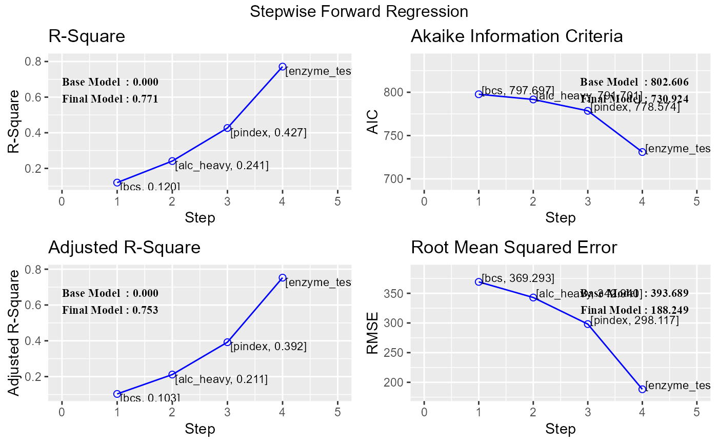
model <- lm(y ~ bcs + alc_heavy + pindex + enzyme_test, data = surgical)
ols_step_forward_p(model, 0.1, hierarchical = TRUE)
#>
#>
#> Stepwise Summary
#> --------------------------------------------------------------------------
#> Step Variable AIC SBC SBIC R2 Adj. R2
#> --------------------------------------------------------------------------
#> 0 Base Model 802.606 806.584 646.746 0.00000 0.00000
#> 1 bcs 797.697 803.664 640.579 0.12010 0.10318
#> 2 alc_heavy 791.701 799.657 633.556 0.24119 0.21144
#> 3 pindex 778.574 788.519 620.215 0.42659 0.39218
#> 4 enzyme_test 730.924 742.858 578.678 0.77136 0.75269
#> --------------------------------------------------------------------------
#>
#> Final Model Output
#> ------------------
#>
#> Model Summary
#> -------------------------------------------------------------------
#> R 0.878 RMSE 197.620
#> R-Squared 0.771 MSE 39053.801
#> Adj. R-Squared 0.753 Coef. Var 28.147
#> Pred R-Squared 0.695 AIC 730.924
#> MAE 140.619 SBC 742.858
#> -------------------------------------------------------------------
#> RMSE: Root Mean Square Error
#> MSE: Mean Square Error
#> MAE: Mean Absolute Error
#> AIC: Akaike Information Criteria
#> SBC: Schwarz Bayesian Criteria
#>
#> ANOVA
#> -----------------------------------------------------------------------
#> Sum of
#> Squares DF Mean Square F Sig.
#> -----------------------------------------------------------------------
#> Regression 6455884.265 4 1613971.066 41.327 0.0000
#> Residual 1913636.272 49 39053.801
#> Total 8369520.537 53
#> -----------------------------------------------------------------------
#>
#> Parameter Estimates
#> ------------------------------------------------------------------------------------------------
#> model Beta Std. Error Std. Beta t Sig lower upper
#> ------------------------------------------------------------------------------------------------
#> (Intercept) -1334.424 180.589 -7.389 0.000 -1697.332 -971.516
#> bcs 81.439 17.781 0.329 4.580 0.000 45.706 117.171
#> alc_heavy 312.777 72.341 0.309 4.324 0.000 167.402 458.152
#> pindex 10.131 1.622 0.431 6.246 0.000 6.871 13.390
#> enzyme_test 11.243 1.308 0.601 8.596 0.000 8.614 13.871
#> ------------------------------------------------------------------------------------------------
#>
# plot
k <- ols_step_forward_p(model, 0.1, hierarchical = TRUE)
plot(k)
 # steps
ols_step_forward_p(model, steps = 3)
#>
#>
#> Stepwise Summary
#> --------------------------------------------------------------------------
#> Step Variable AIC SBC SBIC R2 Adj. R2
#> --------------------------------------------------------------------------
#> 0 Base Model 802.606 806.584 646.746 0.00000 0.00000
#> 1 enzyme_test 782.629 788.596 626.125 0.33435 0.32154
#> 2 bcs 766.271 774.226 609.778 0.52619 0.50761
#> 3 pindex 746.376 756.320 591.430 0.68413 0.66518
#> --------------------------------------------------------------------------
#>
#> Final Model Output
#> ------------------
#>
#> Model Summary
#> -------------------------------------------------------------------
#> R 0.827 RMSE 229.944
#> R-Squared 0.684 MSE 52874.027
#> Adj. R-Squared 0.665 Coef. Var 32.751
#> Pred R-Squared 0.598 AIC 746.376
#> MAE 160.398 SBC 756.320
#> -------------------------------------------------------------------
#> RMSE: Root Mean Square Error
#> MSE: Mean Square Error
#> MAE: Mean Absolute Error
#> AIC: Akaike Information Criteria
#> SBC: Schwarz Bayesian Criteria
#>
#> ANOVA
#> -----------------------------------------------------------------------
#> Sum of
#> Squares DF Mean Square F Sig.
#> -----------------------------------------------------------------------
#> Regression 5725819.203 3 1908606.401 36.097 0.0000
#> Residual 2643701.335 50 52874.027
#> Total 8369520.537 53
#> -----------------------------------------------------------------------
#>
#> Parameter Estimates
#> ------------------------------------------------------------------------------------------------
#> model Beta Std. Error Std. Beta t Sig lower upper
#> ------------------------------------------------------------------------------------------------
#> (Intercept) -1410.847 209.118 -6.747 0.000 -1830.873 -990.821
#> enzyme_test 12.128 1.503 0.649 8.069 0.000 9.109 15.147
#> bcs 101.054 20.005 0.408 5.052 0.000 60.873 141.234
#> pindex 9.382 1.876 0.399 5.000 0.000 5.613 13.151
#> ------------------------------------------------------------------------------------------------
#>